
In this tutorial, you will learn how to transpose in Excel.
A vertical range of cells is converted into a horizontal range, or vice versa, via the TRANSPOSE function. It is necessary to input the TRANSPOSE function as an array formula in a range that has the same number of rows and columns as the source range does.
Once ready, we’ll get started by utilizing real-world examples to show you how to transpose in Excel.
Table of Contents
Anatomy of TRANSPOSE Function
The TRANSPOSE function syntax has the following argument: =TRANSPOSE(array)
Transpose Cells
Before we begin we will need a group of data to be used to transpose in Excel.
Step 1
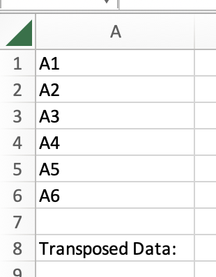
First, you need to have a clean and tidy group of data to work with.
Step 2
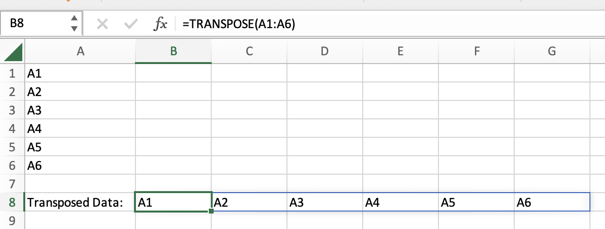
To transpose, simply use the TRANSPOSE function as the following =TRANSPOSE(A1:A6).

Step 3
Once you are done, your Excel will look like this.
Summary
That’s all there is to it. You are welcome to copy the example spreadsheet below to see how it is done. The most crucial lesson is to enjoy yourself while doing it.
In this tutorial, I covered how to transpose in Excel.