In this tutorial, you will learn how to create a crosstab in Excel.
A crosstab query arranges the results by two sets of values—one set on the side of the datasheet and the other set across the top—after calculating a sum, average, or other aggregate function.
Once ready, we’ll start by utilizing real-world examples to show you how to create a crosstab in Excel.
Table of Contents
Create a Crosstab in Excel
Before we begin we will need a group of data to create a crosstab in Excel.
Step 1
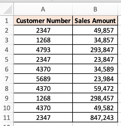
First, you need to have a clean and tidy group of data.
Step 2
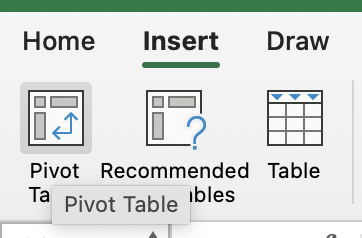
In this example, we will create a crosstab to sum up the same customer numbers to show the total sales incurred from one customer. To do so, we first need to select the entire data group, select “Insert” then select “Pivot Table”.
Step 3
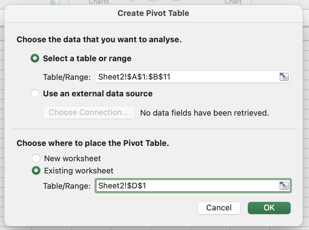
Once you clicked to create a Pivot Table, a pop-up will appear, you can then select whether you want to create the Pivot Table in your existing excel sheet or a new sheet.
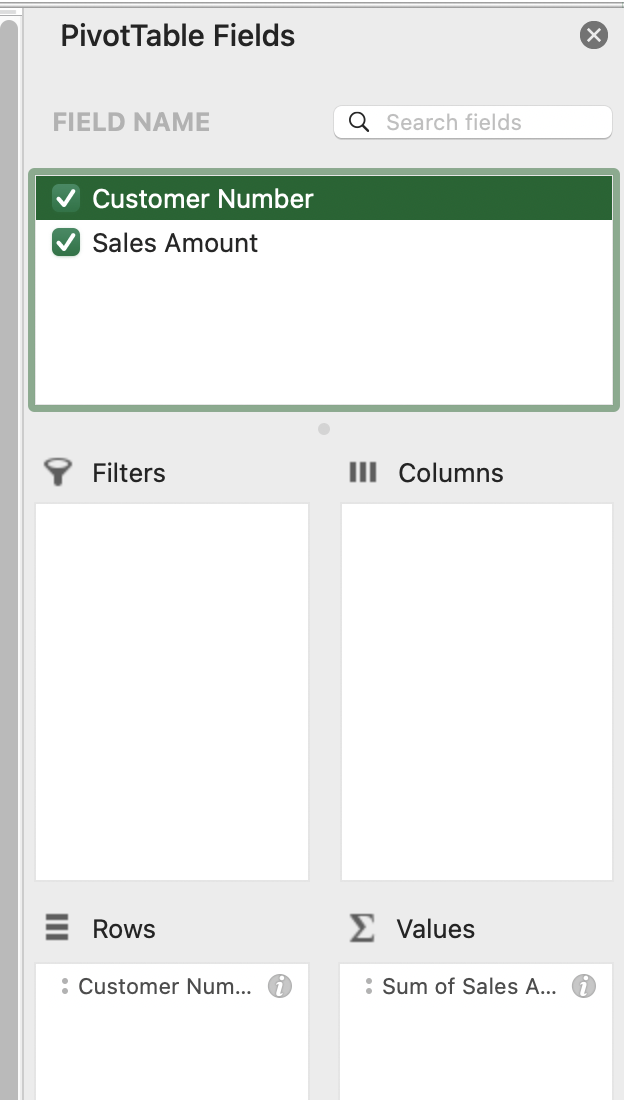
Step 4
In the PivotTable Fields, we will then select the “Customer Number” to “Rows” and “Sales Amount” to “Value”.
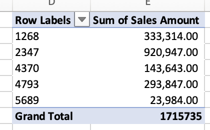
Step 5
Once you are done, your Crosstab will look like this.