
If you’re looking for a way to calculate your GPA using Excel, look no further!
This easy-to-follow guide will show you how to do just that.
Plus, you can use this method to track your grades over time and see how they’ve changed.
So get started today and improve your academic performance!
Table of Contents
How to Calculate GPA in Excel
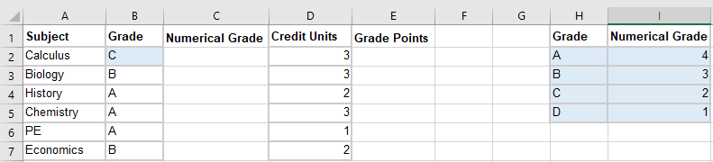
Since Google Sheets and Excel have close to the same functions, we will use the same dataset for this breakdown of steps.
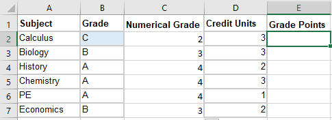
This dataset has the letter grade, credit units, and a reference table.
The methods for calculating GPA are also relatively similar.
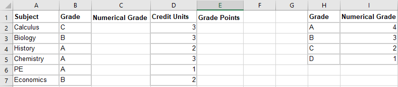
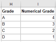
Step 1. Create a reference table
This table should consist of the letter grade and its respective numerical grade.
You can refer to this table later when you want to convert the grades to their numerical counterparts. Your table should look like this:
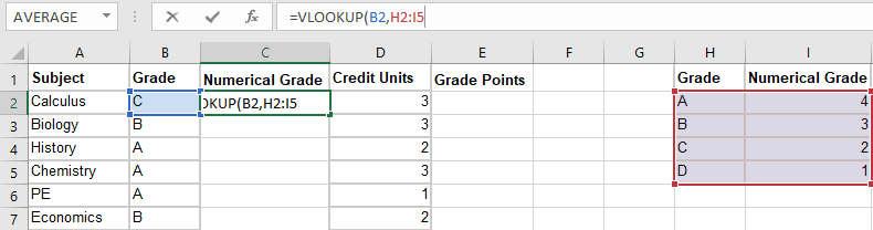
Step 2. Obtain numerical grade using the VLOOKUP formula
Now you have to convert the letter grade to its numerical equivalent.
You can now use the table you created in the previous step as a reference.
Step 2.1. Locate coordinates of the first letter grade (B2) and coordinates of the table (H2:I5) or the cell range.
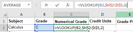
Step 2.2. Click the corresponding cell for the numerical grade and input the following formula into the formula bar initially:
=VLOOKUP(B2,H2:I5…
Step 2.3. Once you finish typing the reference table’s cell range, click the F4 button on your keyboard.
The $ symbol indicates that the values are now made absolute.

Step 2.4. Then, add a comma before typing the number 2.
The number 2 signifies that you will take the data from the second column of the table.
Of course, add a close parenthesis to end the formula.
You should be left with the following final formula:
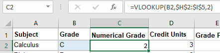
=VLOOKUP(B2,$H$2:$I$5,2)
Step 2.5. Press “ENTER” on your keyboard to apply the formula.
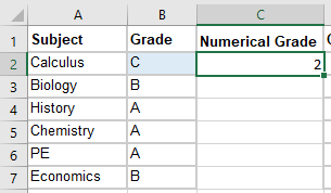
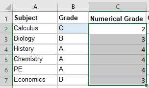
Step 2.6. Apply the VLOOKUP formula to the rest of the cells
Drag the fill handle from the first cell down to the last cell.
The fill handle is the green square at the bottom right corner of a selected cell.
Note: You’ll know when you’re hovering on the correct area if your cursor turns into a plus symbol.
Step 3. Multiply Numerical Grade and Credit Units
Step 3.1. Select the first cell of the column designated for the grade points
Step 3.2. Input the following formula into the formula bar: =C2*D2
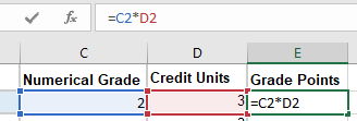
This multiplies the cells that contain the numerical grade and credit units for the first subject, Calculus.
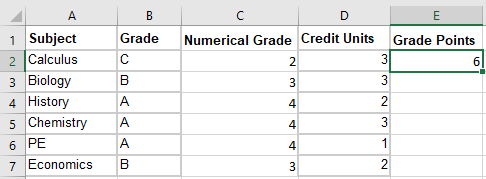
Click “Enter”.
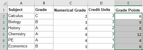
Step 3.3. Apply the formula to the remaining cells using the fill handle.
By now, you know that the fill handle is the green square at the lower right portion of the selected cell.
Drag the fill handle from the first cell down to the last.
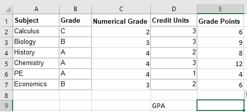
Step 4. Calculate the Grade Point Average (GPA)
Step 4.1. Click the cell where you want the GPA to appear.
The selected cell should have a dark green border.
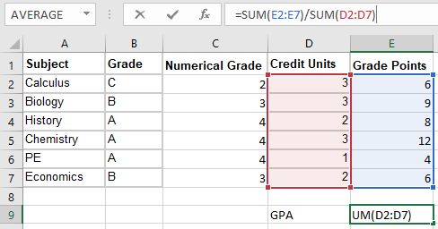
Step 4.2. Divide the sum of the Grade Points cell range (E2:E7) by the sum of the Credit Units cell range (D2:D7)
Therefore, you have to input the following formula into the formula bar:
=SUM(E2:E7)/SUM(D2:D7)
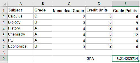
Step 4.3. Click “Enter” on your keyboard.
Doing this should automatically show the GPA on the cell you selected.
Summary
That’s the end of this tutorial.
We hope this article helps you learn how to calculate GPA in Excel