
In this tutorial, you will learn how to use conditional formatting in Excel.
To conditionally format cells in a range that contain duplicate text, unique text, and text that is the same as text you define, use the Quick Analysis tool. Even better, you can conditionally format a row based on the text that appears in one of its cells.
Once ready, we’ll get started by utilizing real-world examples to show you how to use conditional formatting in Excel.
Table of Contents
Use Conditional Formatting in Excel
Before we begin we will need a group of data to be used to use conditional formatting in Excel.
Step 1
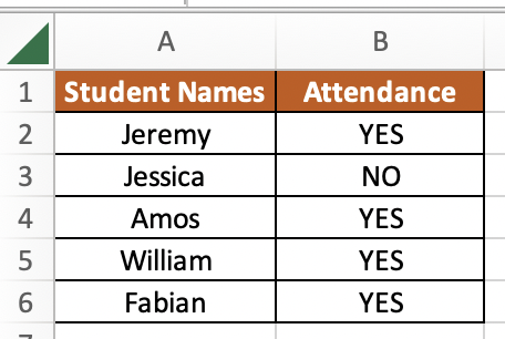
First, you need to have a clean and tidy group of data to work with.
Step 2
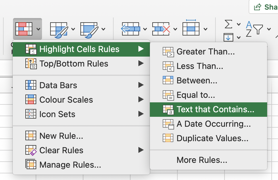
In this example, we want to know to highlight the cells with the word “YES”. to do so, we will select the entire data group, then select ‘Home’, then select ‘Conditional formatting’, then select ‘Highlight Cells Rules’, and select ‘Text that Contains’.
Step 3
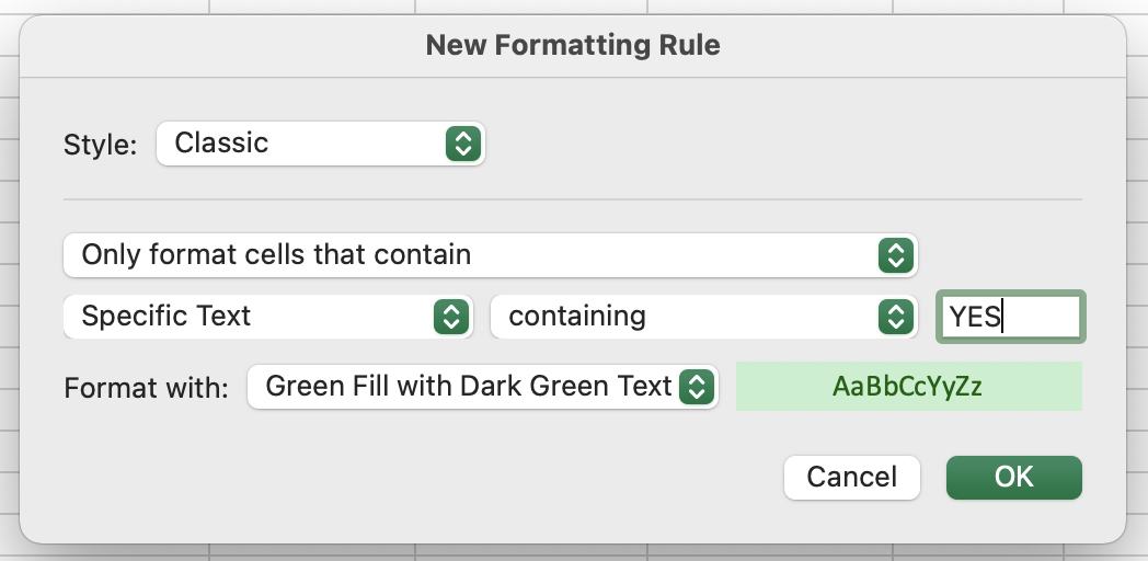
A pop-up box will appear, we will then customize the color we want to fill the cells containing the word ‘YES’ with green.
Step 4
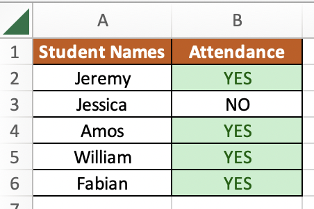
Once you press ‘OK’, your cells will look like this.
Summary
That’s all there is to it. You are welcome to copy the example spreadsheet below to see how it is done. The most crucial lesson is to enjoy yourself while doing it.
In this tutorial, I covered how to use conditional formatting in Excel.