In this tutorial, you will learn how to filter data horizontally in Excel.
You can freely choose to show or hide numerous entries in a dataset by using filters. When discussing a horizontal filter, you can see the worksheet’s filtered sections. You must practice it because it is not a trait that is built-in, so keep that in mind. In contrast to vertical filters, this filter filters your columns rather than your rows to view the information you require.
A horizontal filter can be created in a variety of methods. Excel’s FILTER feature must be used to apply a filter horizontally. You can use the filter feature to filter a table using the criteria you specify. Once the table has been located, you can use the row’s name or even define the filtering criteria.
Once you are ready, we can start by using real-life scenarios to help you understand how to filter data horizontally in Excel.
Table of Contents
Anatomy of FILTER Function
=FILTER(array, include, [if_empty])
You can use the FILTER function to filter a variety of data according to parameters that you specify.
SUMIF Cells Not Equal to Value in Excel
Before we begin we will need a group of data to be used to filter data horizontally in Excel.
Step 1
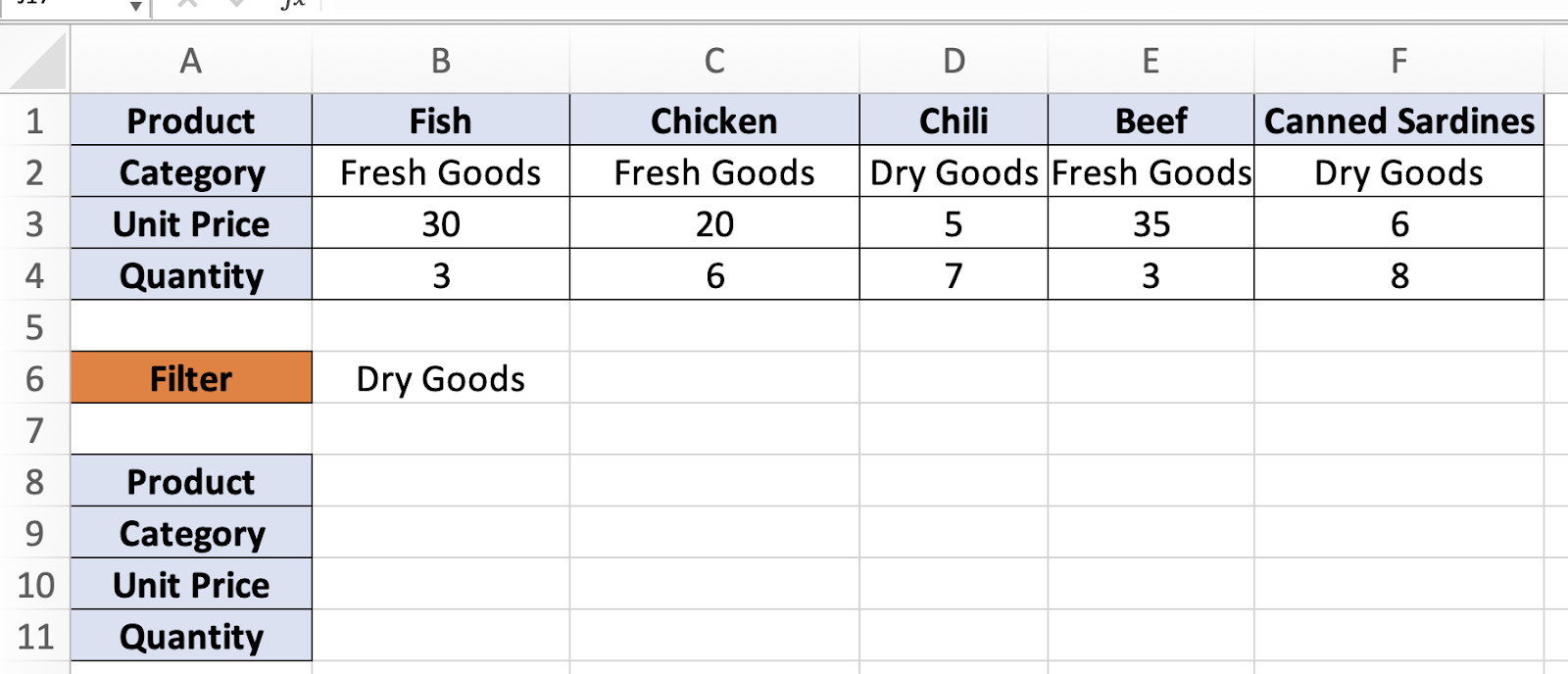
First, you need to have a clean and tidy group of data to work with.
Step 2
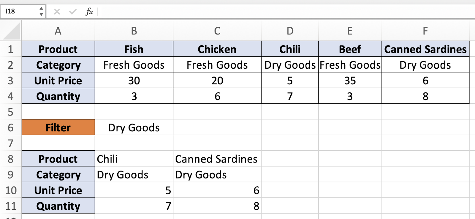
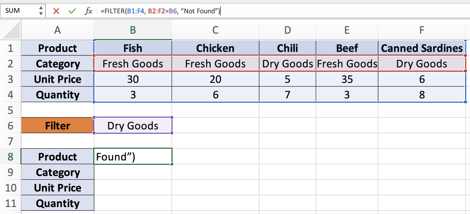
In this example, we want to filter the ‘Dry Goods’ products. To do that, we will insert the following formula =FILTER(B1:F4, B2:F2=B6, “Not Found”).
Step 3
Once we are done, you will be able to filter data horizontally.