How To Calculate Ratio in Google Sheets

Google Sheets is a powerful online spreadsheet application that you can use to perform complex calculations.

In this tutorial, we will teach you how to calculate ratios in Google Sheets.

We will also provide some tips on how to make the process easier and more efficient.

Let’s get started!

How to Calculate Ratio in Google Sheets

You may not know it, but we do ratios or fractions almost in our daily lives from the moment you wake up.

When you make your cup of coffee, you use the ratio where a certain teaspoon of coffee will require a certain amount of sugar and creamer.

The formula for that will look like coffee:sugar:creamer.

Changing the amount of coffee will also change the sugar and creamer you put in. Interesting, isn’t it?

People widely use ratios to have the same outcome, even if the quantity differs. Sometimes, when the numbers are too large or there are many data sets, it is hard to compute them mentally.

It is where learning how to calculate ratios in Google Sheets and Excel will come in handy.

How To Calculate Ratio in Google Sheets

Google Sheets is a great application when you want to edit anywhere and on any device.

Furthermore, it allows multiple people to edit simultaneously.

Here are the steps to calculate the ratio in Google Sheets.

Step 1

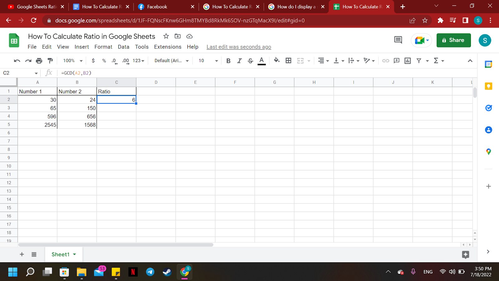
Find the Greatest Common Denominator or GCD between the two numbers with the formula =GCD(A2,B2).

You will use the same GCD formula for the second number in the ratio.

Step 2

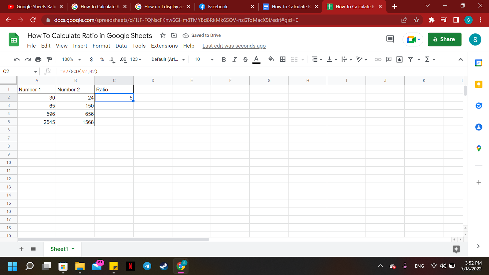
Let’s find the ratio for Number 1 using the formula =A2/GCD(A2,B2).

Step 3

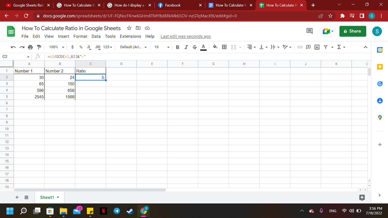
To add the ratio symbol ‘:,’ you must add it to the formula.

The formula then will become =A2/GCD(A2,B2)&”:”.

Step 4

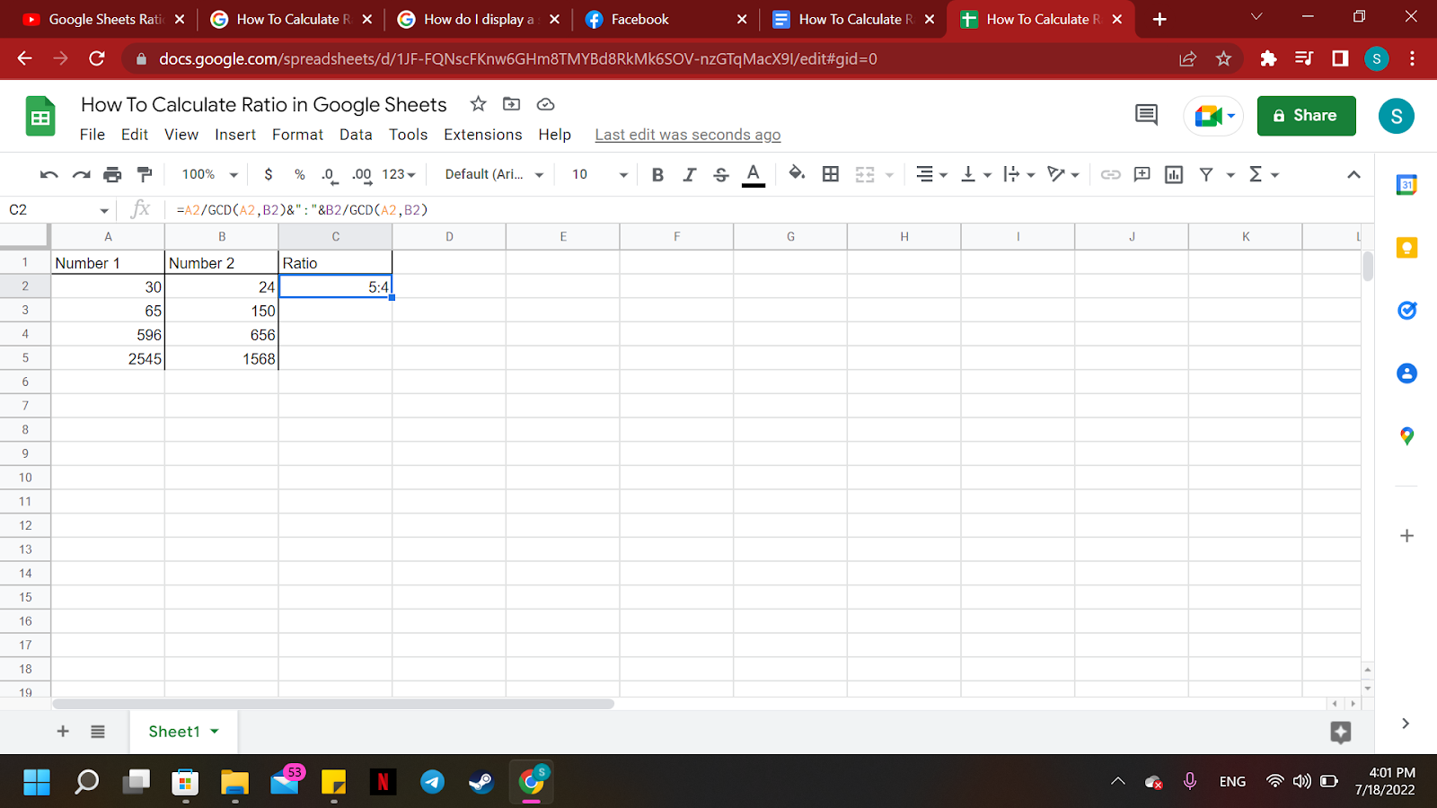
To finish the ratio while having the symbol, you will need to add another ‘&’ to separate them.

The additional formula to find the 2nd number is the same as the formula used to find the 1st number of the ratio.

However, you will replace the “A2” before the dividend with “B2.” The final formula will be =A2/GCD(A2,B2)&”:”&B2/GCD(A2,B2).

Step 5

If you have a list of numbers that needs a ratio, you don’t have to do the long formula one by one.

All you need to do is hold the left click to the little box on the bottom-right corner of the first ratio.

Step 6

Drag it down until the last pair of numbers.

Running dots will appear to guide you while you are dragging down your cursor.

Step 7

Once you release the left click, all the ratios will show up simultaneously.

And there you go!

You now have the ratios of all the numbers you need in the Google Sheets.

Summary

That’s the end of this tutorial.

We hope this article helps you learn how to calculate Ratio in Google Sheets.