
Google Sheets is a great tool for calculating percentages.
In this tutorial, you’ll learn how to use the percentage function in Google Sheets to quickly and easily calculate percentages.
You’ll also learn how to use the percent difference and percent of total functions.
Let’s get started!
Table of Contents
How to Calculate Percentage in Google Sheets
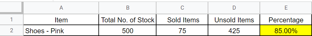
To calculate the percentage of unsold items, we need first to deduct the number of ‘Sold’ items from the ‘Total No. of Stock.’
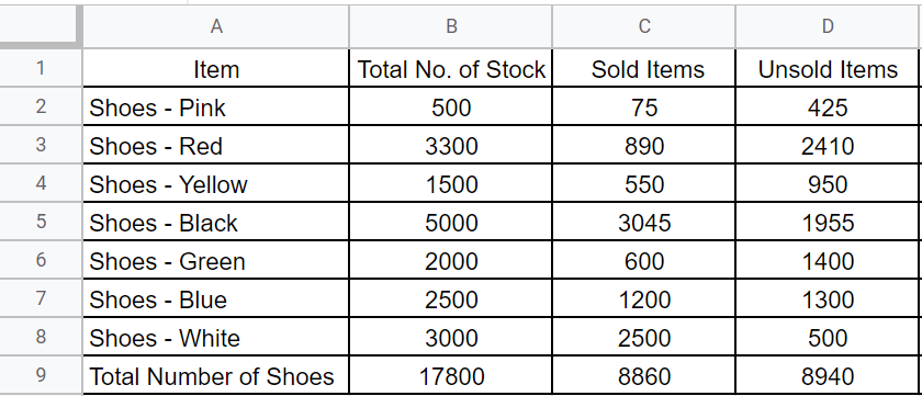
Using the data of the ‘Unsold Items,’ we can now compute the percentage in Google Sheets.
Method 1. Using Basic Formula
Step 1. Determine the data that you need to compute the percentage.
In this example, we will use the data under ‘Unsold Items’ as the ‘Part’ and the ‘Total Number of Stock’ as the ‘Total or Whole Part.’
Step 2. Use the Basic Percentage Formula.
To get the percentage, use the formula below:
Part of the Whole / Whole = Percentage
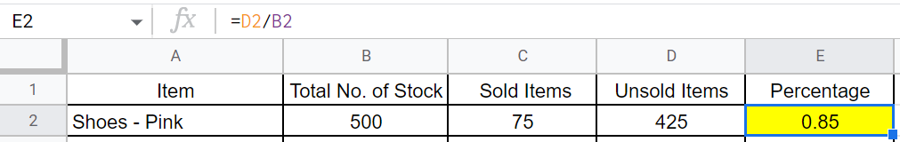
Step 3. Determine the cell where you want to put the returning value.
For this example, the returning value will be keyed in E cells.
Step 4. Substitute the formula with the actual data.
This means that when we calculate the percentage in Google Sheets and Excel, the formula will look like this:
=D2/B2
Step 5. Press the ‘Enter’ key.
How you set up your Google Sheets spreadsheet may show a percentage result like the one below.
Don’t worry if the returning value shows in decimals. You can easily change this by following the steps below.
Step 5.1 Highlight the returning cell’s value.
Step 5.2 Click the percent sign ‘%’ in the toolbar menu.
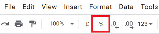
After you click the percent sign, the spreadsheet will automatically change the format of the returning value. It will now show like this:
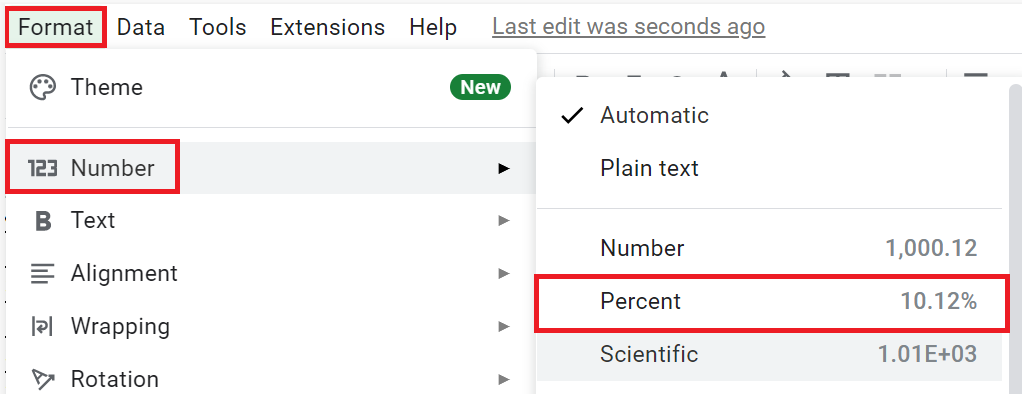
If your spreadsheet does not display any ‘%’ sign, you may follow the following steps to convert the format from decimals to percent.
Step 5.2.1 Click ‘Format’ > ‘Number’ > ‘Percent’.
Step 5.3 Copy the returning value to the remaining cells.
Copying the returning value will automatically copy the formula and the format too.
You don’t need to manually put the procedure in each cell and manually highlight and click the percent sign.
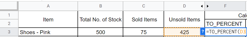
Method 2. Use the TO_PERCENT function.
If you are a fan of using Google Sheet functions, you may use the ‘TO_PERCENT’ to automatically generate the returning value as a percent.
Step 1. Select a cell for the returning value.
Step 2. Substitute the formula with actual data.
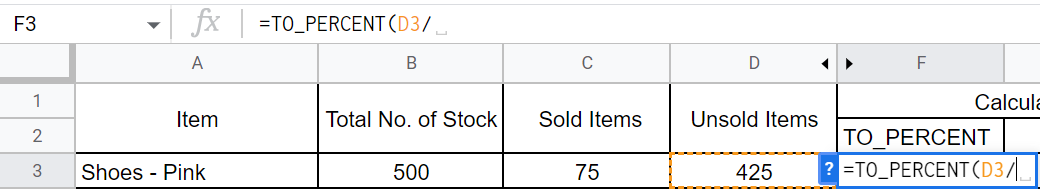
=TO_PERCENT(Part/Total)
So, the formula above should now look like this:
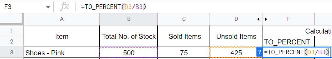
=TO_PERCENT(D3/B3)
D3 represents the Unsold Items, and B3 represents the Total No. of Stock.
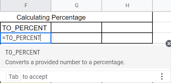
Step 3. Key in the ‘= TO_PERCENT’ formula in the designated cell.
Always start the formula with an equal sign ‘=’ when writing it. Writing the equal sign before typing in the formula lets the spreadsheet identify that you are writing formula and not a text.
Step 4. Input the ‘Part’ cell range.
Note: The ‘Part’ and the ‘Total’ cell ranges must be enclosed in an open parenthesis.
Step 5. Key in the Slash symbol ‘/.’
The slash symbol also represents division. In Google Sheets, this symbol divides a number from a whole.
Step 6. Add the ‘Total’ cell followed by a closing parenthesis.
This is now what the formula looks like in your spreadsheet.
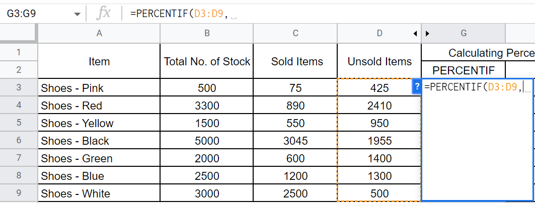
Method 3. Use the ‘PERCENTIF’ function.
The PERCENTIF function in Google Sheets is mainly used for more complex percentage computation.
Some of these computations include specific conditions that may seem impossible for some to calculate percentages in Google Sheets and Excel.
However, to successfully get the returning value, you need to ensure that you are correctly writing the function’s syntax.
PERCENTIF(range, criteria)
Where:
Range refers to the cell range of the data you need to work on
Criteria refer to a condition, text, or cell
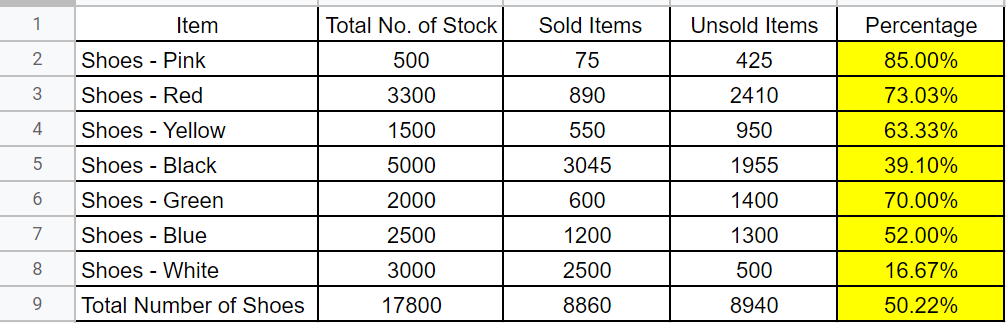
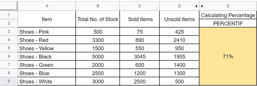
Using the same given data, we will get the percentage of the number of items that have unsold stocks greater than 500.
Step 1. Select the cell for the returning value.
Step 2. Key in the PERCENTIF function.
In this formula, the D3:D9 represents the cell of the data which we will get the condition from.
While “>500″ is the condition that we will set to complete the function in calculating the percentage of the number of unsold items greater than 500.
=PERCENTIF(D3:D9,”>500″)
Start writing with the function and the cell range like the one below.
Step 3. Add the condition.
Since we will be computing the percentage of the unsold items greater than 500, the condition will look like “>500”.
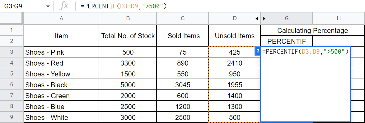
Step 4. Press’ Enter.’
Summary
That’s the end of this tutorial. We hope this article helps you learn how to calculate Percentage in Google Sheets.