
Percentages can be used in a variety of ways, from calculating discounts and tips to comparing proportions.
In this blog post we will show you how to calculate percentages in Excel.
The steps are easy to follow and we have provided screenshots so that you can easily follow along.
After reading this blog post, you will know how to perform basic calculations using percentages in Excel.
So let’s get started!
Table of Contents
How to Calculate Percentage in Excel
Don’t you know that you can also quickly calculate percentages in Excel?
Here are some of the most commonly used methods that you can use to calculate percentages in Excel.
Method 1. Using Basic Multiplication Formula
This method is mainly used for smaller data sets that don’t need a complex formula.
When using this method, all you need to do is multiply the percent by the base number.
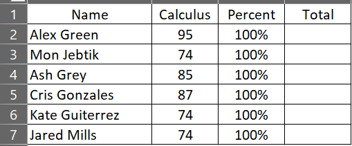
For example, a teacher needs to compute the students’ grades to determine who passed and failed on specific subjects.
From the given an example below, we will determine how many students pass the subject.
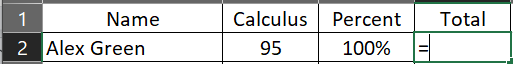
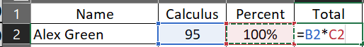
Step 1. Start writing the formula with an equal sign (=).
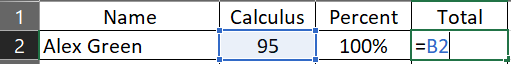
Step 2. Select the cell range of the base number you want to get the percentage from.
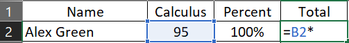
Step 3. Add the asterisk (*).
The asterisk serves as the multiplication symbol in our formula.
Step 4. Select the percent cell range to complete the formula.
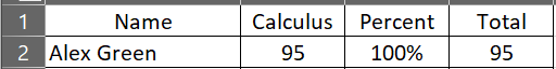
Step 5. Press’ Enter’.
Excel will automatically generate the result once you press the Enter key.
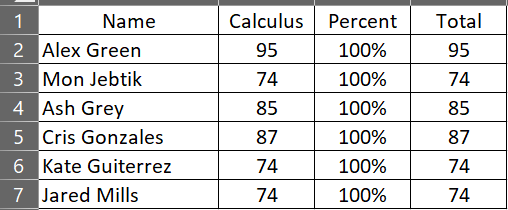
Step 6. Copy the result to other cells.
Copying and pasting the result to the other cells will automatically generate the returning value as a percent.
Method 2. Use the SUMIF function.
Another method to calculate percentages in Excel is the SUMIF function, which adds the numbers that fall under one criterion.
For example, we need to calculate the percentage of specific meat.
To get the total percentage of that specific meat, we need to use the SUMIF function below.
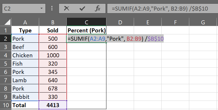
=SUMIF(range, criteria, sum_range) / total
Take note:
The range refers to the number of cells we need to add to make up the base number from which we will get the percentage.
The criteria refer to the specific item or product you want to get the percentage of.
Sum_range refers to the cell range of all the items or products listed.
Total refers to the total number of items or products.
Step 1. Write the function.
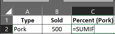
Always keep in mind, whether you are writing in Excel or Google Sheets, the function should start with an equal sign (=).
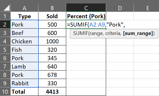
Step 2. Add the cell range.
This cell range refers to the criteria or number of items or products we need to summarize.
Step 2. Following the sequence on the pop-up, add the criteria.
For this example, our criteria are pork.
You can add the word ‘pork’ in the formula or specifically create a cell for the criteria and use it to substitute the criteria in the formula.
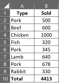
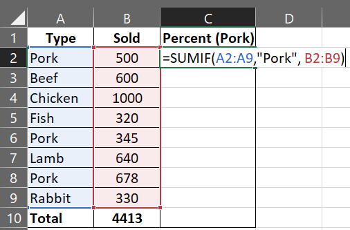
Step 3. Add the cell range that you need to get the returning value from.
The example below covers cells B2 to B9.
Though we need to get the percentage of the pork sold, we still need the numbers of the other items to determine the total number of items sold.
From here, we will be able to get the percentage of the pork sold from the whole product sold.
Step 4. Key in the divide symbol (/).
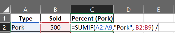
Step 5. Input the cell range for the total number of items.
The sample below has dollar signs ($) written before and after the letter B.
The dollar sign locks the cell range to ensure that the reference stays as is when you drag and drop the formula to other cells.
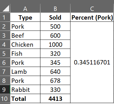
Step 6. Press the ‘Enter’ key to get the returning value.
Summary
That’s the end of this tutorial. We hope this article helps you learn how to calculate Percentage in Excel