
Looking to calculate interest in Google Sheets?
You’ve come to the right place! In this tutorial, we’ll show you how to do it using different formulas.
We’ll also provide a few tips on how to choose the right one for your needs.
So whether you’re a student or a working professional, read on for all the steps you need to get the job done.
Table of Contents
How to Calculate Interest in Google Sheets
Calculating interest is of significance in the world of accounting or banking.
As we all know, interest is an amount of money gained from a principal amount.
This amount is usually based on a specified rate of increase.
There are two types of interests.
First, we have simple interests, which from the name are simply from the principal amount with a fixed rate and time.
Meanwhile, compound interest is the amount gained from the principal and the interests accumulated from it after a certain period of compounding.
In this article, the steps for calculating both simple and compound interest are broken down and discussed.
Calculating Interest In Google Sheets
Method 1. Calculating Simple Interest
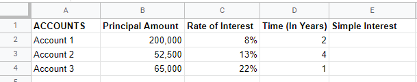
Calculating simple interest involves only three essential values, namely the principal amount, yearly interest rate, and time in years.
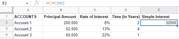
Suppose this is the dataset you will be using.
You have to calculate the simple interest for these three accounts.
Step 1. Load up your sheet

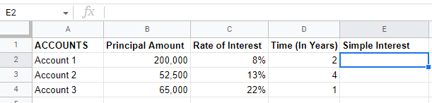
Step 2. Click the cell where you want the simple interest to appear
The selected cell should appear with a blue border.
Since you already have a table prepared, you can start with the simple interest for the 1st account.
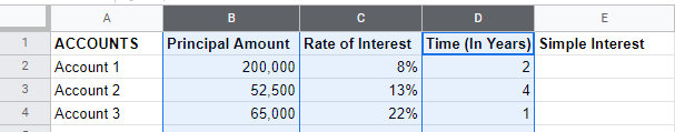
Step 3. Locate the coordinates of the cells
Check the coordinates of the cells with the relevant data. For this example, all data are in columns B, C, and D.
The cells you want to calculate are B2, C2, and D2.
Step 4. Input the simple interest formula
The formula for principal interest is:
A = P x r x t
Where: A is the simple interest
P is the principal
r is the rate per year
t is the time in years.
Thus, based on this and cell coordinates, the formula you have to input into the formula bar is:
=B2*C2*D2
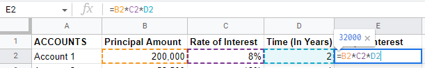
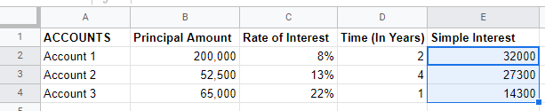
Step 5. Click “Enter” on your keyboard
Clicking the “Enter” button on your keyboard should automatically show the simple interest in the selected cell.
Step 6. Copy the formula to the remaining cells
You can do this by dragging the fill handle to the last cell.
The find handle is a blue square in the selected cell’s lower right corner.
Method 2. Calculating Compound Interest
For compound interests, the formula is more complex compared to simple interests.
The data needed, however, are relatively similar.
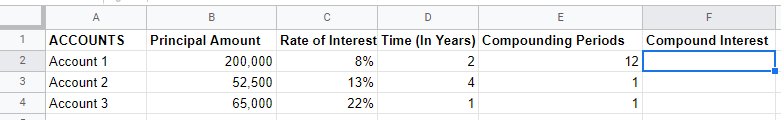
The only addition is the amount of compounding periods in a year. The number of periods is usually one of the three: yearly (1), monthly (12), or daily (365).
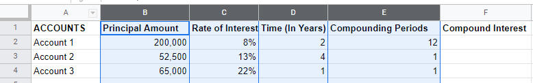
Suppose this is the dataset you will use.
Step 1. Load up your sheet
Step 2. Click the cell where you want the compound interest to appear
The selected cell should appear with a blue border.
Since you already have a table prepared, you can begin with the compound interest for the 1st account.
Step 3. Locate the coordinates of the cells
Check the coordinates of the cells with the relevant data.
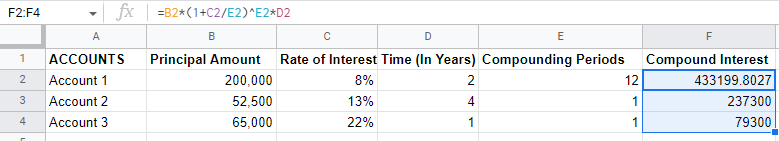
For this example, all data are in columns B, C, D, and E.
The cells you want to calculate are B2, C2, D2, and E2.
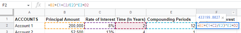
Step 4. Input the compound interest formula
This is where it gets tricky.
Compound interest has a more complex formula which is:
A = P(1 + r/n)nt
Where: A is the compound interest
P is the principal
r is the yearly interest rate
n is the number of times compounded each year
t is the time in years
Based on this and the cell coordinates established earlier, the formula you have to input into the formula bar is:
=B2*(1+C2/E2)^E2*D2
Note: * is the multiplication symbol, / is the division symbol, ^ turns the succeeding values into an exponent
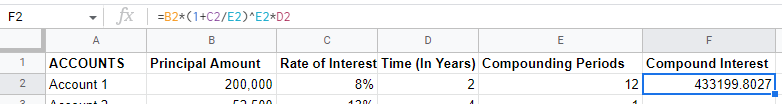
Step 5. Click “Enter” on your keyboard
Clicking the “Enter” button on your keyboard should automatically show the compound interest in the selected cell.
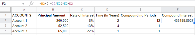
Step 6. Copy the formula to the remaining cells
You can do this by dragging the fill handle to the last cell.
The find handle is a blue square in the selected cell’s lower right corner.
Summary
That’s the end of this tutorial.
We hope this article helps you learn how to calculate Interest in Google Sheets.