
In order to calculate interest in Excel, you’ll need to know the basics of how to use Excel formulas.
After that, it’s just a matter of using the right formula for the type of interest being calculated.
Here are some tips on how to get started.
Table of Contents
How to Calculate Interest in Excel
Method 1. Calculating Simple Interest
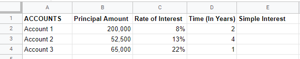
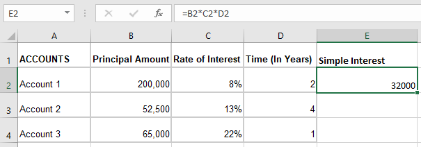
We will use this dataset for Excel.
Suppose you have to calculate the simple interest for these three accounts.
Calculating simple interest involves only three essential values, namely the principal amount, yearly interest rate, and time in years.
Step 1. Open your workbook

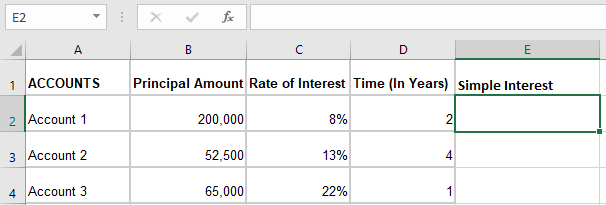
Step 2. Click the cell where you want the simple interest to appear
The selected cell should appear with a dark green border.
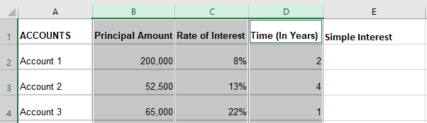
Step 3. Locate the coordinates of the cells
Locate the cells with relevant data. For this example, all data are in columns B, C, and D.
The cells you want to calculate are B2, C2, and D2.
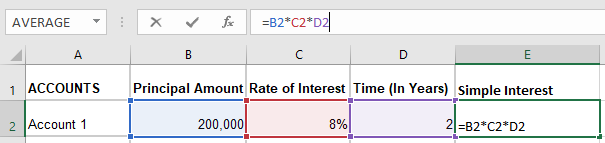
Step 4. Input the simple interest formula
The formula for principal interest is:
A = P x r x t
Where: A is the simple interest
P is the principal
r is the rate per year
t is the time in years.
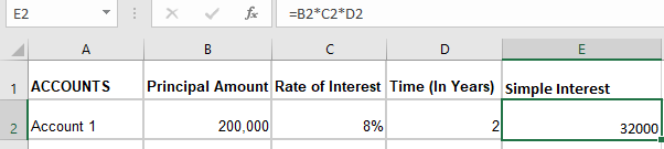
Thus, based on this and cell coordinates, the formula you have to input into the formula bar is:
=B2*C2*D2
Step 5. Click “Enter” on your keyboard
Clicking the “Enter” button on your keyboard should automatically show the simple interest in the selected cell.
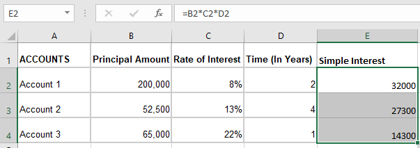
Step 6. Copy the formula to the remaining cells
You can do this by dragging the fill handle to the last cell.
The find handle is a dark green square in the selected cell’s bottom right part.
Method 2. Calculating Compound Interest
The formula for compound interest is a tad bit tricky compared to simple interests.
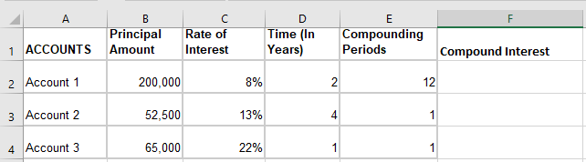
The data needed, however, are relatively similar. This time, there is an amount of compounding periods in a year.
The number of periods is usually yearly (1), monthly (12), or daily (365). Suppose this is the dataset you will use.
Step 1. Open your workbook
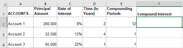
Step 2. Click the cell where you want the compound interest to appear
The selected cell should appear with a dark green border.
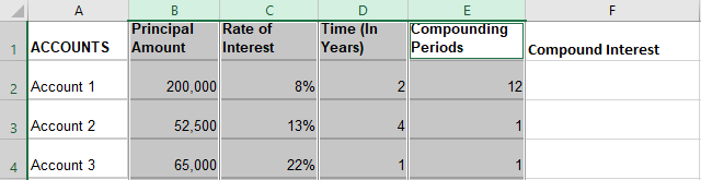
Step 3. Locate the coordinates of the cells
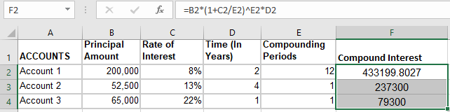
Locate the cells with relevant data. For this example, all data are in columns B, C, D, and E. The cells you want to calculate are B2, C2, D2, and E2.
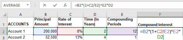
Step 4. Input the compound interest formula
Compound interest has a trickier formula which is:
A = P(1 + r/n)nt
Where: A is the compound interest
P is the principal
r is the yearly interest rate
n is the number of times compounded each year
t is the time in years
Based on this and the cell coordinates established earlier, the formula you have to input into the formula bar is:
=B2*(1+C2/E2)^E2*D2
Note: * is the multiplication symbol, / is the division symbol, ^ turns the succeeding values into an exponent
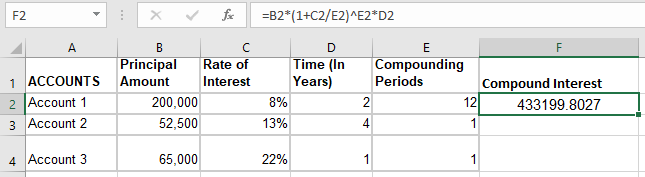
Step 5. Click “Enter” on your keyboard
Clicking the “Enter” button on your keyboard should automatically show the compound interest in the selected cell.

Step 6. Copy the formula to the remaining cells
You can do this by dragging the fill handle to the last cell.
The find handle is a dark green square in the selected cell’s bottom right part.
Summary
That’s the end of this tutorial.
We hope this article helps you learn how to calculate Interest in Excel