
Are you looking for a way to calculate your GPA without having to use a traditional calculator?
If so, you’re in luck!
In this blog post, we will show you how to do it using Google Sheets.
So whether you are a student or just need to keep track of your grades, this method is definitely worth checking out.
Let’s get started!
Table of Contents
How to Calculate GPA in Google Sheets
One of the tasks users can perform with the famous spreadsheet applications, Google Sheets and Excel, is computing for GPA or grade point average.
A GPA is usually a numerical grade multiplied by the respective credit units.
The product is divided by the total number of units to get the average.
Calculating GPA is a task most commonly done by professors or teachers.
It’s not easy to perform manually, especially for classes with many students.
Thankfully, Google Sheets and Excel have them covered.
How to Calculate GPA in Google Sheets
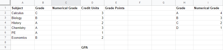
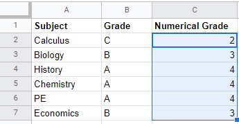
Suppose this is the dataset you are going to calculate.
You already have each class’s grade and the number of credit units.
You now need the equivalent numerical grade, the grade point, and finally, the average/GPA.
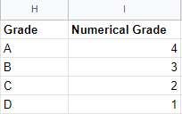
Step 1. Create a reference table
This table will be used as a reference for later when you want to convert the grades to their numerical counterparts.
Your table should look like this:
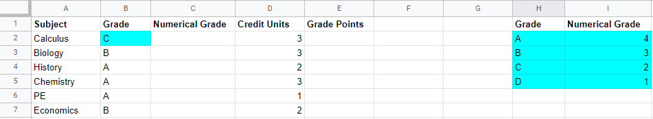
Step 2. Obtain numerical grade using the VLOOKUP formula
It’s time for you to convert the letter grade to its numerical equivalent.
You will now use the table you created in the previous step as a reference.
Step 2.1. Take note of the coordinates of the first letter grade (B2) and coordinates of the table (H2:I5) or the cell range.
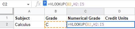
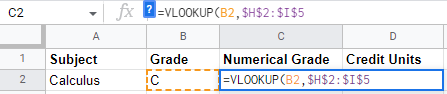
Step 2.2. Input the following formula into the formula bar:
=VLOOKUP(B2,H2:I5…
Step 2.3. Once you finish typing the reference table’s cell range, press the F4 button on your keyboard.
Doing this will make the values absolute (signified by the $ symbol).
Step 2.4. Then, add a comma before typing the number 2. The number 2 signifies that you will take the data from the second column of the table.
Of course, add a close parenthesis to end the formula.
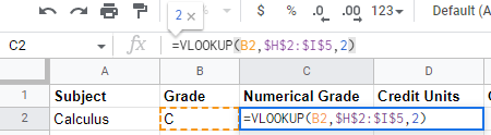
Thus. the final formula should be:
=VLOOKUP(B2,$H$2:$I$5,2)
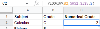
Step 2.5. Click “ENTER” on your keyboard to apply the formula.
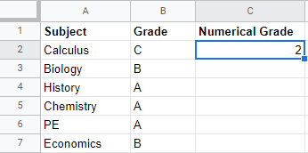
Step 2.6. Apply the VLOOKUP formula to the rest of the cells
Drag the blue square found on the first cell’s lower right portion down to the column’s last cell.
This blue square is known as the fill handle.
Note: You’ll know when you’re hovering on the correct area if your cursor turns into a plus symbol.
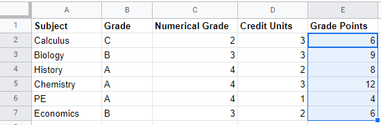
Step 3. Multiply Numerical Grade and Credit Units
Step 3.1. Select the first cell of the column designated for the grade points
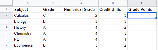
Step 3.2. Input the following formula into the formula bar: =C2*D2
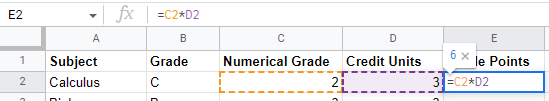
This multiplies the cells that contain the numerical grade and credit units for the first subject, Calculus. Click “Enter”.
Step 3.3. Apply the formula to the remaining cells using the fill handle. As mentioned earlier, the fill handle is the blue square at the bottom right corner of a selected cell.
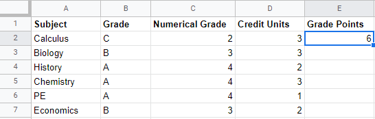
Drag the fill handle from the first cell down to the last.
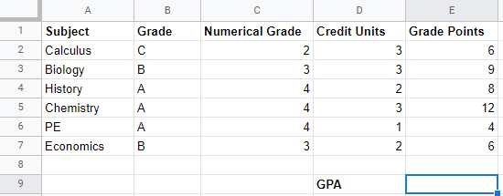
Step 4. Calculate the Grade Point Average (GPA)
Step 4.1. Click the cell where you want the GPA to appear. The selected cell should have a blue border.
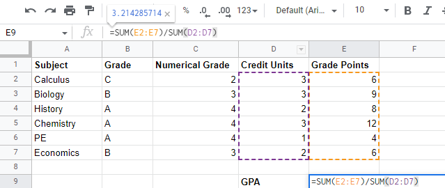
Step 4.2. Divide the sum of the Grade Points cell range (E2:E7) by the sum of the Credit Units cell range (D2:D7)
Therefore, you have to input the following formula into the formula bar:
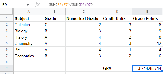
=SUM(E2:E7)/SUM(D2:D7)
Step 4.3. Click “Enter” on your keyboard. Doing this should automatically show the GPA on the cell you selected.
Summary
That’s the end of this tutorial.
We hope this article helps you learn how to calculate GPA in Google Sheets.